Predictive Analysis of Parkinson's Disease Using Machine Learning
Abstract
Background
Parkinson's disease is one of the major nerve disorders that affect physical movement, which leads to tremors in individuals above 50 years of age. The affected individual will face walking and speech difficulties. According to the Parkinson Foundation, about 0.3% of the human population is affected across the globe. WHO reported that Parkinson’s disease affects a large population of about 10 million people worldwide. Patients left untreated with timely medication will lead to fatal neurological functional disorders. Due to environmental changes, food habits, and lifestyle, the number of people affected by this disease is gradually increasing.
Aim
This study aimed to predict Parkinson’s disease using speech signals and applying various AI techniques and identify the research gaps to improve the treatment efficiency with respect to detection rate and cost.
Objective
The objective of this study was to efficiently predict Parkinson’s disease using shallow learning AI algorithms, such as Support Vector Machine, XGBoost, and Multilayer Perceptron Deep Neural Networks algorithms under limited patient data with the aid of efficient feature selection algorithms like Principal Component Analysis (PCA) and Analysis of Variance (ANOVA) for selecting the most distinguishing features.
Methods
The dataset containing speech samples was obtained from the UCI repository, which included samples from 188 individuals. The data preprocessing involved the application of the Synthetic Minority Oversampling Technique (SMOTE), and a comparative study of PCA and ANOVA was carried out to select the optimal features. Then, the algorithms SVM, XGBoost, and DNN were employed.
Result
When PCA was used for dimensionality reduction, DNN and XGBoost demonstrated higher accuracy, but SVM exhibited lower runtime. On the other hand, when ANOVA was applied for dimensionality reduction, all three algorithms showed good accuracy, with DNN proving more efficient for a smaller number of features.
Conclusion
All the algorithms, when combined with both dimensionality reduction techniques, exhibited an average accuracy of 97%. In comparison, the ANOVA feature selection technique led to shorter training times compared to PCA. However, PCA resulted in a comparatively fewer number of optimal features for all three algorithms, which resulted in the trade-off between the number of optimal features and training times. Therefore, to increase the efficiency of decision-making for improved disease detection, there is a need to explore multimodal and multi-objective approaches.
1. INTRODUCTION
Health is the most important aspect of humans. According to WHO, the health zone is expanding at an expeditious pace compared to the financial system. Many countries have legal and legislative frameworks for health care. Out-of-pocket expenditure by individuals has experienced a significant growth in health [1]. As more people understand the significance of health, there is a great demand for healthcare professionals, but unfortunately, the increase in demand has surpassed the supply by multiple folds, leading to limited and increased costs of health care. So, the best alternative for this is to opt for digital diagnosis and treatment for diseases/ailments.
With the greater advancements in technology, presently, the diagnosis and treatment through technology has not just brought down health care expenses but has also been significantly faster and more accurate. Artificial intelligence/machine learning plays a vital role in this sector [2]. The early success of technology-based diagnosis/treatments has led to an increase in better technology development, particularly in specialized medical domains that were once thought to require only human expertise.
Certain forms of Parkinsonism tend to be hereditary, and several could be related to peculiar genetic mutations. Many researchers agree that Parkinsonism is a consequence of a mixture of genetic and hormonal causes, like subjection to contamination. If the world's population lives longer, chronic illnesses, such as Parkinson's disease, are projected to become more prevalent [3]. Adults over the age of 60 are more likely to be diagnosed with Parkinson’s disease. The proportion of patients with Parkinson's disease was projected to be 4.1 million and 4.6 million in 2005, but that trend is estimated to more than double by 2029 to between 8.5 million and 9.2 million.
Artificial intelligence (AI) is a synthesized intelligence for machines to mimic human behaviour or human intelligence. Automation is capable of predictable and repetitive tasks because it lacks the intelligence part, which is a key component of the decision-making process. Due to the advancement in technology, machines are now capable of making decisions in a simple scenario without human intervention, which is because of machine-based learning, which is unsupervised learning, the key to making decisions [4] and also in complex situations, where a lot of things are to be considered when making decisions, requiring human intervention, which is supervised learning for the machine.
The main aim of this study is to predict Parkinson’s disease by considering the dominating features of voice samples and applying various AI techniques like SVM, XGBoost, and DNN to identify the research gaps and to improve the treatment efficiency with respect to detection rate and cost.
Speech dataset plays a vital role in Parkinson's Disease (PD) research and diagnosis. The early signs of the disease can be predicted. The detection of changes in the normal speech pattern, such as slurred speech, reduced speech volume, and difficulty with articulation, helps in the detection of disease. The changes in pitch, volume, speech rate, and other vocal characteristics are difficult to identify by clinical observations, which can be determined effortlessly using AI techniques. Analysing the speech samples is less stressful than diagnostic methods like blood tests and brain imaging.
This study is structured as follows: section 2 presents the related work, which describes the disease characteristics and also summaries the usage of various algorithms like SVM, XGBoost, and DNN for prediction and classification of real-world problems like travel time prediction, task classifier, audio classifier, etc. Section 3 provides a description of the dataset taken from the UCI repository and data preprocessing with a description of the algorithm used in the work. Section 4 discusses the experiment, analysis, and methodologies used in this study, and the last section discusses enhancement in the prediction of Parkinson’s disease.
2. LITERATURE OVERVIEW
This section gives an overview of Parkinson’s disease and the uses of Support Vector Machines (SVM), Deep Neural Networks (DNN), and Extreme Boosting Algorithms (XGBoost) in various applications.
DeMaagd et al. [5] gave an overview of Parkinson’s disease. This illness was first found by Dr. James Parkinson. It was discovered in 1817. This disease is also known as “shaking palsy”. It is characterised by both nonmotor and motor qualities. Motor symptoms are due to the loss of neurons. The nonmotor symptoms include sleep disorders, cognitive changes, and depression. It is the most common neurodegenerative disease, commonly found in elderly citizens of America. The disease is also linked to mortality. Additionally, it is associated with genetic mutations.
Dennis [6] conducted a study on Parkinson’s disease that describes the neuropathology of the disease. The disease is characterized by posture instability, rigidity, bradykinesia, and tremor [7]. A summary from cell biology and animal studies gives a molecular pathology of this disease [8]. Individuals affected by this disease experience symptoms of autopsy or other pathologic symptoms, such as atrophy and cerebrovascular disease. In this disease, the nervous system is also affected.
Shin et al. [9] proposed an automatic task classifying system using SVM for mobile devices. The dataset used was collected using the Amazon Mechanical Turk Platform (MTurk), which offers a structure for the collection of huge data sets. A tenfold cross-validation approach utilizing SVM was applied to thirty-two tasks to assess classification accuracy. This method quantified precision and memorized value for each task. On considering declassification among analogous tasks, the accuracy ranged from 82% to 99%, making task classifiers eligible to be used in subordinate services. Voice calls were passed on to a server system that used the Sphinx speech recognition system and ran a task divider. The acquired speech was converted to text and was given to the task classifier that classified it as a feasible task and reverted to the user's mobile, where the task launcher performed an apparent task.
Selvaraj [10] worked on an acoustic guidance system for hearing-impaired people that uses support vector machine classifiers to categorise the audio signals. This was done in two steps. First, input audio was subjected to wavelet transform to find the feature of the audio signal; next, it was processed by an SVM classifier. This study offered (14+2L) dimension feature vectors for audio ordering and grouping, which were composed of perceptual features and frequency cepstral coefficients. The Fourier transform mapped audio signals to the frequency domain from the time domain. The output of this phase was given as input to SVM for classifying different sounds. This technique, by applying SVM, demonstrated an accuracy above 90%, and classification errors were minimized to 3%.
Hardiyanti et al. [11] introduced a human activity classifier based on data from sensors using SVM. The dataset used was gathered from an accelerometer and gyroscope embedded in smartphones with Android applications. This device was positioned on the right foot of the human for about 30 seconds to measure the values. Human activities can be classified into two types: the first type is simple activity, such as doing only one work at a time. The second type is complex activities, where the activity is carried out for a long duration of time [12]. Using the accelerometer, the degree of tilt of the smartphone was measured, whereas the gyroscope governed the motion [13]. To reduce the classification errors, the SVM ensemble technique was used. The test data constituted 30% of the dataset and was balanced with the training data. The use of SVM resulted in an accuracy of 99.1%, specificity of 98.7%, and sensitivity of 99.6%.
Lavanya [14] described a predictive method for forecasting tragedies by utilizing a vast collection of historical data using SVM. Information was collected by the National Transport Safety Board (NTSB), which has a five to eight-year record of aircraft accidents. This data was pre-processed in order to fill in the missing fields and remove the unconnected data. To source the recent data, data filtering was done. A clean dataset was obtained after the process of pre-processing. Next, for classification, the polynomial kernel function of SVM was used, which formed a multi-dimensional hyper-plane that separated data as the cause of accidents and did not cause accidents. The accuracy that was achieved through SVM was 96.27%.
Kusal [15] proposed a system to predict the travel hours of a tour in a taxi service using the XGBoost regression algorithm. Accurate prediction of travel time facilitated decision-making for riders and drivers. Travel time is the total time passengers have to be seated in the vehicle until they reach their destination [16]. Travel time that is predicted during the start of the journey is known as static time, which is not subjected to changes and does not predict traffic jams or waiting time [17]. XGBoost was used for multiple scenarios with scarcer necessities. The dataset used in the study was collected using FOIL. In data pre-processing, GPS pickup and drop-off coordinates were considered. Anonymous trips were removed from datasets [18]. The authors concluded that XGBoost has the ability to decrease time transmission projection error when compared to other models.
Matousek et al. [19] introduced a system to identify Glottal Closure Instants (GCIs) in speech signals using XGBoost. GCIs in speech signals are peaks in voice. The speech data was collected from the recordings of speeches in the author's workspace, which consisted of both male and female voices. XGBoost uses a technique called boosting, which is repeated until no improvements can be made. The performance was evaluated by parameters precision (P), F1, and AUC. To select important features, a feature selection algorithm was used. The preferred quantity of features was validated through a 10-fold cross-validation method. XGBoost gave an accuracy of F1=98.55% and an AUC of 99.90%.
Panagopoulos [20] presented their work on forecasting the behaviour of drivers if driving is dangerous using the XGBoost algorithm. The risks, such as aggressive and distracted driving, are challenging to measure. These factors were predicted by short-term calculations. The algorithm was fed with a collection of vehicular and emotional variables. The dataset used was SIM1; it contained data based on the driving styles of the driver. The system monitored the driving patterns of the drivers and alerted them when usual patterns were not found. Sensorimotor disruptions were tracked. The features that were extracted were statistical, correlative, temporal, structural, and spectral. The algorithm worked on the concept of a timing window. For the results evaluation, at meta-prediction and fast track levels, 5-fold cross-validation was applied. The AUC for both the predictions was 84%.
Tan [21] described a method of classification of music style systems using XGBoost. To extract features like tumbrel texture, pitch content, and rhythmic content, a jSymbolic tool was used. Mainly, eight features were customized, which, on the whole described melody music. The dataset was collected from five melody composers: Haydn, Beethoven, Schubert, Bach, and Mozart. This study compared XGBoost and BPNN algorithms. XGBoost demonstrated the highest value in view of accuracy, precision, recall, F-measure and AUC.
Wang and Han [22] proposed a speech recognition system built on deep neural networks (DNN). This system operated on a combination of a shallow neural network along with DNN. The datasets used in this experiment were a recording of fifty speakers. Five emotions were considered, namely neutral, anger, sadness, surprise, and joy. Moreover, in this study, 4 hidden layers were used to extract emotional attributes. The first step was to collect the samples and make quantifications, framing, and sampling. The next step was to establish a training sample set, followed by treating the trained deep belief network on subsets. Lastly, the results were acquired. Considering all five emotions, the average accuracy of the system was 89.8%.
Amroun [23] submitted a work on the recall of individual jobs in an unrestricted environment based on DNN. Using a grid with an intelligent object, the following activities were tracked: sitting, walking, lying down, and standing. The smart objects that were used were smartphones, smartwatches, and a remote control. These devices formed three layers of DNN. The experiment was carried out on seven people, and the duration was one week. To record a person’s activity, three IP cameras were fixed with respect to various places in the room and a local server was used to store the captured activity [24]. The training sets were divided into fine-tuning and pre-training. DNN gave an average accuracy of 98.53%.
Almakky [25] introduced a system for text localisation in biomedical figures using DNN. The dataset used was DeTEXT. It consisted of 500 biomedical images and 9308 regions of text. Three hundred images were used for testing and 100 for validation. The input image was first remodelled into a single-channel image. The obtained rebuilt image was black-white in nature. The system was built based on unsupervised learning and was built such that the required image size was maintained. Transformation functions, such as colour inverse, random rotation, random crops, scaling, and random-sized crops, were used on images. The training dataset was extracted using ground truth for bounding boxes. The images of a bigger scale were reduced to 200 * 200 sized images. By applying the threshold function, the binary image was reconstructed. Lastly, the noise filter was added to identify the noise. The precision was 62%, and recall was 91%.
Feng et al. [26] presented a system for predicting material defects using DNN. The dataset used had 487 data points. The solidification defects were predicted. Initially, DNN was adjusted with biases and weights, which were approximate to the global optimal solution and helped in fine-tuning. PCA was used to reduce the noise and data dimensions; out of 487 data points, 324 were taken as training sets, while the remaining 163 were test sets. SVM and DNN structures were used. The system consisted of 21 neurons, hidden neurons, and one output neuron. Transformation functions were used for the hidden layer. The training accuracy was increased to 0.98 from 0.73, and testing accuracy increased to 0.86 from 0.67.
Yang [27] described a system to predict the airline share market using DNN to estimate the modest capacity of aircraft in the market of aeronautics. The trade share evaluation model used the DNN. Asian aviation market dataset was considered for the experiment [28]. The attributes considered to predict the share market were: day type, alliance, codeshare, tin size, number of segments (nbrseg), departure time (deptime), time circuitity, distance circuitity, arrival time (arrtime), and the number of stops. The computation of share market was computed on a weekly basis for the flights that were not planned at the same timings. Logistic regression was used to calculate the market share. The mean error when DNN was used was 2.4 *10-19; when compared to logistics, it was 5.2 * 10 -5. The absolute mean error on using DNN was 0.02, and when using logistics, it was 0.05.
The literature survey summarizes the SVM algorithm used for task classifier and audio classifier, the XGBoost algorithm used for prediction of travelled time and identification of speech signals, and the DNN algorithm used for tracking various physical activities, material defects, and airline prediction share market. The proposed system gave a higher accuracy when the number of features was increased for these algorithms.
3. METHODOLOGY
In this section, various algorithms used for analysing Parkinson's disease are described. In this study, the most well-known methods like Support Vector Machine, Deep Neural Networks, and XGBoost were used for the analysis.
AI has been an area of interest in terms of human competencies in the aspects of machines. We humans have certain physical and mental limitations; almost all human beings have great human capabilities that are limited by our own intellect or physical limitations. Human capabilities, such as problem-solving skills, are a gift. However, these abilities are hard to pass on or to be learned by fellow humans. In spite of teaching/learning skill sets, we sometimes fail to recreate or reproduce similar or better results every time. On the contrary, machines are far more capable of handling predictable and repetitive kinds of tasks.
A neural network is a network of neurons which are in several millions. These interconnected neurons help in communication, information retrieval, information processing, etc. ANN is an evaluating technique, which draws to imitates the approach of the human brain to examine and operate the details. An Artificial Neural Network is similar to a biological neuron but in terms of technology. ANNs have self-learning capabilities.
In the case of an ANN, the process executes, where the model learns from the training data by adjusting its parameters based on the inputs and expected outputs. The network learns to identify vision or text. During the learning phase, the connections aggregate the received outputs and compare them with the desired end product. The conflict between results is corrected by the backpropagation method. The network works backward in this manner, making a contrast between the actual and needed outcomes less probable. The unit adjusts the weights of the interconnected input units to modify the relationships between components until an error is minimized.
A Recurrent Neural Network (RNN) is a part of ANNs, where the connections between nodes are in a temporary sequence. It forms a directed graph that depicts the network’s temporary dynamic behaviour. RNNs obtained out of feedforward neural networks have varying term series of feeds. They use memory to process, which applies to projects like unclassified, joined handwriting, or speech recognition.
3.1. Dataset Description
The dataset was taken from the Kaggle database, and data was collected from the UCI Machine Learning Repository [29]. Data was collected from 252 total test subjects, out of which 188 were suffering from Parkinson's disease, which is represented with the class status ‘1’ and the remaining 64 were healthy individuals, represented as status ‘0’. The statistical features obtained in the dataset were based on the domain-level features obtained from the test subjects presented in Table 1. A total of 756 samples and 753 features were extracted from the test subjects. The data was collected by setting a microphone at 44.1 KHz to record the speeches of the participants. Table 2 presents the dataset distribution.
| 1. Baseline Features | 5. Vocal Fold |
|---|---|
| 2. Intensity Parameters | 6. MFCC |
| 3. Formant Frequencies | 7. Wavelet Features |
| 4. Bandwidth Parameters | 8. TQWT Features |
| Class | Number of Samples |
|---|---|
| 0 (Healthy) | 192 |
| 1 (Diseased) | 564 |
3.2. Data Preprocessing
A significant imbalance was observed in the class distribution of the dataset. Hence, in order to obtain better accuracy from the ML algorithms, we began by balancing the distribution through the Synthetic Minority Oversampling Technique (SMOTE). Table 3 gives an overview of the balanced dataset.
| Class | Number of Samples |
|---|---|
| 0 (Healthy) | 450 |
| 1 (Diseased) | 450 |
3.3. Optimizing the Complexity of the Model
3.3.1. Principal Component Analysis
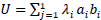
The collected data was huge, which could lead to the diminution of the model’s accuracy. To reduce the complexity of the model, feature selection and extraction were employed. By maintaining the relevant information, the features of data were reduced to lower dimensional by using Principal Component Analysis (PCA). PCA is used when it is necessary to reduce a set of variables in order to make them independent of one another. There are a series of steps followed to use PCA. First, Eqs. (1-3) were used for dimension transformation matrix U by considering a sample vector y and mapping it to a new j-dimensional feature subspace, which has a lesser dimension than the original e-dimensional feature space.
 |
(1) |
 |
(2) |
 |
(3) |
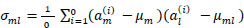
The second step was to create a covariance matrix of dimension e of the dataset. The covariance between two features a_m and a_l on the population is represented by Eq. (4).
 |
(4) |
Where, µm and µl are sample means of features i and l.
Next, the variance ratio is represented by Eq. (5), which is as follows:
 |
(5) |
 |
Finally, the projection matrix was computed by transforming the sample to PCA subspace using the matrix dot product.
3.3.2. Analysis of Variance
Analysis of Variance (ANOVA) is a statistical method used to analyse the differences among groups and their variation. It is the technique to extract the features that contribute significantly to the prediction of disease. ANOVA works by examining the ratio of variance between groups to the variance within groups. When used for feature selection, it assesses whether the mean differences between the target variable's classes (e.g., labels) are statistically significant based on each feature. A high F-value from ANOVA indicates a feature that provides significant discriminatory power between the classes, making it a good candidate for selection. ANOVA is particularly useful for datasets with numerical features and categorical target variables. For instance, in medical diagnosis, ANOVA can help identify which biomarkers are most associated with the presence or absence of a disease.
3.4. Exploring Supervised Learning Techniques
3.4.1. Support Vector Machine
This is one of the well-received supervised machine learning algorithms that works effectively on small data sets rather than large datasets. SVM is mainly used to solve the problems which come under classification. Support Vector Machines (SVMs) have been used as powerful tools to solve classification and regression problems. SVM aims to find a hyperplane that models the training data based on their class labels. This hyperplane is mapped to a higher-dimensional space, where structural risk is minimized. Legacy quadratic programming algorithms have been proposed, but massive matrix storage for these algorithms and calculation of expensive matrix operations are required. To avoid such problems, such as Sequential Minimal Optimization (SMO), which is more convenient to implement, an agile, iterative algorithm is chosen to train SVMs.
There are several advantages of SVM. It works well with a proper separation of margin, and it is more effective in high dimensional, making it memory efficient. Equally, SVM has a few loopholes, such as when the dataset increases, it takes more time and fails to work whenever the dataset consists of noise.
SVM is built on the concept of hyperplane. A line that divides the data into different groups is known as a hyperplane. Eqs. (6 and 7) represent the line as:
 |
(6) |
 |
(7) |
Considering two vectors, I=(x,y) and J=(a,-1), they can be represented by Eq. (8) as:
 |
(8) |
If there are l training samples, where each example a has e dimension and each is labelled as either b=+1 or b=-1, the training data can be written as:
{ai,bi} where i=1,2,……..l, bi € {-1,1}, a € Re
The optimization value can be given by the Eq. (9):
 |
(9) |
The final calculation is represented in Eq. (10) as:
 |
(10) |
3.4.2. XGBoost Algorithm
XGBoost is a machine learning algorithm that can be used on structured data. It works on the concept of decision trees. The different forms of XGBoost are gradient boosting, stochastic, and regularized gradient boosting. These procedures can be used wherever we need to increase the execution speed and model performance. This belongs to the ensemble learning classification of ML algorithms with three subsets, namely bagging, which has two different features that define prediction and training. Next is stacking, which controls output from numerous input features, and finally, boosting, which is applied to trees.
An initial function is considered based on the simplest linear approximation of function f(z), which is represented in Eq. (11).
 |
(11) |
In the above function, b is the prognosis at step (t-1) while (y-b) is the new learner, which has to be added in step (t) for the purpose of minimizing goals.
By using Taylor's Theorem, the function f(z) can be written in the simplest function of ∆z, as shown in Eqs. (12 and 13).
By applying second-order Taylor approximation, we obtained the following equations:
 |
(12) |
 |
(13) |
Where,
gi = ∂y(t-1)l(yi, y(t-1)) and hi = ∂y2(t-1)l(yi, y(t-1))
By eliminating constants, a simple aim can be written using Eq. (14) as:
 |
(14) |
The binary classification with log loss optimization can be written using Eq. (15) as:
 |
(15) |
Where,
 and y is the real label, and q is the probability score.
3.4.3. Deep Neural Networks
A neural network with two or more layers is known as a Deep Neural Network (DNN). It uses sophisticated models to progress data in multifaceted ways. Each layer performs specific tasks like ordering and sorting. It has efficient usage in dealing with unstructured data. They are termed feed-forward nets as they transport data from the input layer to the output layer. We can move behind the previous layer by using backpropagation. To determine the output of a neuron, an activation function is used. It maps the output value between 0 to 1. ReLU activation function is used, which is a linear function supporting all positive values, and the value is zero for all negative values. Eq. (16) presents the function as:
 |
(16) |
Softmax activation function, as shown in Eq. (17), makes a vector of n real values to a vector of n values, which sum to 1. This activation function transforms the values into a range between 0 and 1, enabling them to be interpreted as probabilities.
 |
(17) |
Where, is the input vector, is an element of the input vector, is the standard exponent, and n is the number of classes in multi-class classifiers.
A Multilayer Perceptron (MLP) is a fundamental building block of Deep Neural Networks (DNNs). It is a type of feedforward neural network consisting of an input layer, one or more hidden layers, and an output layer. Each layer is composed of nodes (neurons) that are fully connected to the next layer, making MLPs suitable for supervised learning tasks like classification and regression. The main function of an MLP is to map input data to the desired output by learning patterns through a process of backpropagation and gradient descent.
4. RESULTS
Dimensionality reduction technique PCA was applied to the dataset to select the dominant feature out of 500. The 22 dominant features obtained were also subjected to XGBoost, SVM, and DNN models. All the models were trained with 70% of the data, and the rest were tested. The algorithms were applied by considering 5 different sets of data. In all cases, the XGB algorithm was the most efficient. DNN showed a constant accuracy value of approximately 78%.
Table 4 provides an overview of the results.
Figs. (1 and 2) show the accuracies with respect to the various algorithms used.
| Sl No. | Number of Features | Accuracy Percent of SVM | Accuracy Percent of XGBoost | Accuracy Percent of DNN |
|---|---|---|---|---|
| 1 | 500 | 73.12 | 78.41 | 78.41 |
| 2 | 350 | 72.24 | 78.41 | 77.09 |
| 3 | 200 | 64.31 | 79.29 | 77.09 |
| 4 | 50 | 75.33 | 85.02 | 77.09 |
| 5 | 22 | 76.65 | 84.58 | 77.09 |
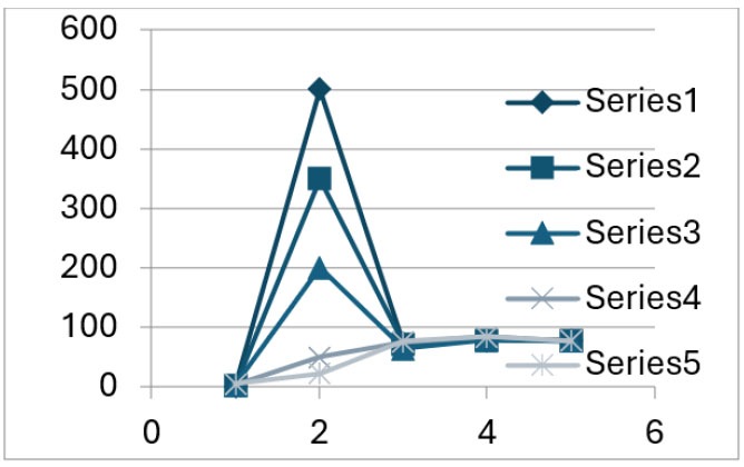
Accuracy vs. machine learning algorithm.
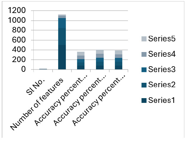
Accuracy vs. machine learning algorithm-2.
5. DISCUSSION
The datasets employed in this study were obtained from the Kaggle [18]. The samples were recorded by positioning a microphone 20 cm away from the source, with voice recordings captured using a 16-bit sound card on a desktop computer at a sampling frequency of 44,100 Hz. To extract the features from the samples, Linear Discriminant Analysis (LDA) was carried out, and then they were stored in the CSV format [18].
The selection of ruling features plays a vital role in the prediction model. Principle Component Analysis (PCA) was carried out on the dataset to obtain the desired number of dominant features. SVM, XGBoost, and DNN models were built and trained using 70% of the data. XGBoost model yielded 85.02 % and 78.41% accuracy for 50 and 500 dominant features, respectively. In the SVM model, 76.65% and 64.31% accuracy were obtained for 22 and 200 principal components, respectively. The neural network was constructed with the softmax activation function applied to both the input and output layers, and multiple hidden dense layers were added with the activation function. The evaluation metric considered in this study was accuracy, where the DNN model yielded a constant accuracy value of approximately 78%.
This study considered important features of the speech signals related to Parkinson’s disease. DNN gave an accuracy of 78%. The disease was detected by incorporating dominant features from over 300,000 voice samples, resulting in high accuracy despite the small dataset size and fewer dimensions. In the future, the system can be developed for large datasets with more dimensions to detect disease with improved accuracy and for more voice modulations considering different datasets and features and by using scans of the diseased person.
6. EXPERIMENTATION, ANALYSIS, AND DISCUSSION
6.1. Dimensionality Reduction
The dataset offered a total of 753 features extracted from the above-mentioned test subjects. Since only a part of the total features were needed for effective classification, we performed dimensionality reduction to select the most discriminating features that were statistically significant for decision-making. We employed the Principal Component Analysis (PCA) and Analysis of Variance (ANOVA).
6.2. Experiments on PCA
In order to reduce the dataset dimension to obtain statistically significant features for improved correlation, PCA extracted a subset of principal components from the total features.
As shown in Fig. (3), it was observed that the SVM algorithm has an approximate optimal performance of 97% for accuracy and detection rate (recall) for the top 140 features extracted by PCA. We further observed that the scores were consistent throughout higher feature counts. The XGBoost algorithm exhibited consistent performance from the top 40 to 500 features, as shown in Fig. (4). Interestingly, after 500 features, the performance dropped significantly to 0, necessitating further investigation.
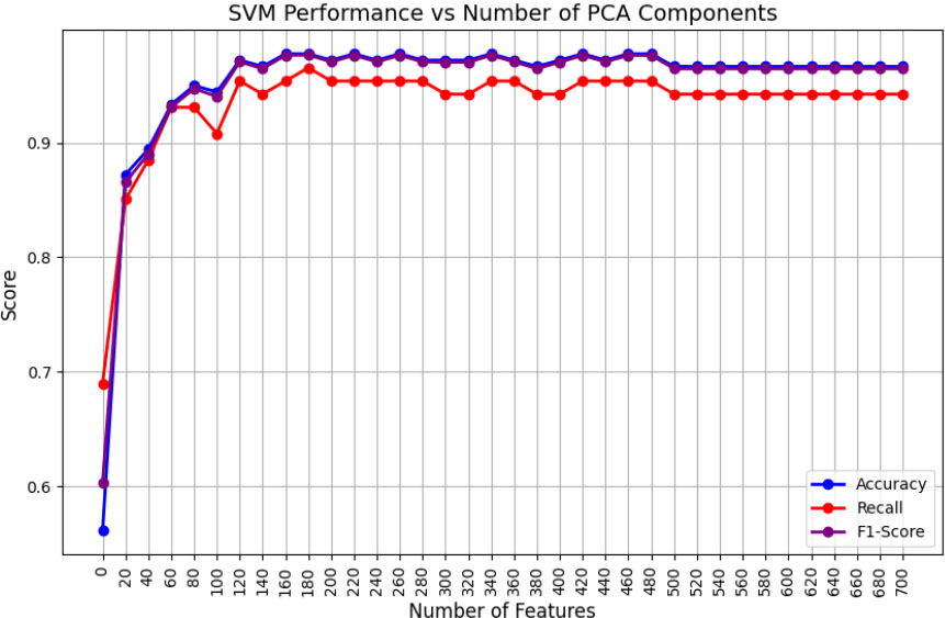
Performance of SVM vs. the number of features with PCA.
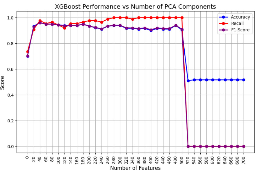
Performance of XGBoost vs. the number of features with PCA.
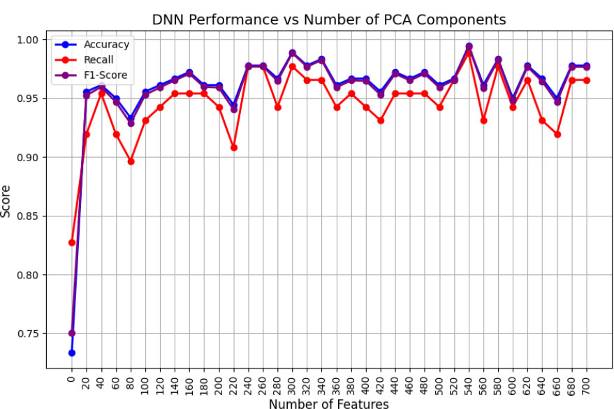
Performance of DNN vs. the number of features with PCA.
However, the DNN considered for the experiments was a Multilayer Perceptron Neural Network algorithm with user-defined features, making it a shallow learner with 50 hidden layers and 100 neurons in each layer. DNN demonstrated an optimal performance, as shown in Fig. (5). The top 40 features achieved an overall performance of 99%, which was made possible by the efficient use of the backpropagation technique.
Tables 5-7 present the detailed parameters of the respective algorithms deployed.
| Parameter | Value |
|---|---|
| Scaler | StandardScaler() |
| Classifier | SVC(kernel='rbf', max_iter=200) |
| Optimal Features | 140 |
| Training Time (seconds) | 44 |
| Parameter | Value |
|---|---|
| Scaler | StandardScaler() |
| Classifier | XGBClassifier(use_label_encoder=False, eval_metric='logloss') |
| Optimal Features | 40 |
| Training Time (seconds) | 98 |
| Parameter | Value |
|---|---|
| Scaler | StandardScaler() |
| Classifier | MLPClassifier(hidden_layer_sizes=(100, 50),max_iter=500) |
| Optimal Features | 40 |
| Training Time (seconds) | 104 |
Upon comparing the three algorithms, it was found that although SVM considered a larger number of features than the other two algorithms, it demonstrated superior performance with relatively shorter training times. This is attributed to the nonlinearity of the RBF kernel, even with an increased number of convergence iterations. Moreover, due to the time-consuming operation of backpropagation, DNN took more time, even for fewer optimal features. Finally, XGBoost demonstrated a similar performance to DNN.
6.3. Experiments on ANOVA
We employed ANOVA, which is a univariate feature selection technique to achieve dimensionality reduction, obtaining optimal performances with a minimal number of distinguishing features. After applying ANOVA, we observed a significant improvement in the classifier performances.
It was observed that the SVM algorithm has an overall optimal performance close to 96% for the top 300 features extracted by ANOVA, as shown in Fig. (6). Further observations indicated that the metrics were consistent. Similarly, the XGBoost algorithm demonstrated a saturated optimal performance of 97.78% accuracy, with a significant improvement in the detection rate of 95.4%, as shown in Fig. (7). However, DNN demonstrated optimal performances at 100 features, where the accuracy and F1_Score were 96% approximately and recall was 94.44%, as shown in Fig. (8). Tables 8-10 present the detailed parameters of the respective algorithms deployed.
The DNN algorithm demonstrated a superior overall performance of 96% compared to the other two algorithms, using only 100 features. This was attributed to the high-variance features selected by ANOVA, along with an adequate number of hidden layer neurons to capture them independently.
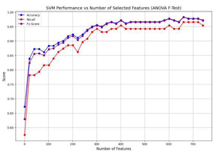
Performance of SVM vs. the number of features with ANOVA.
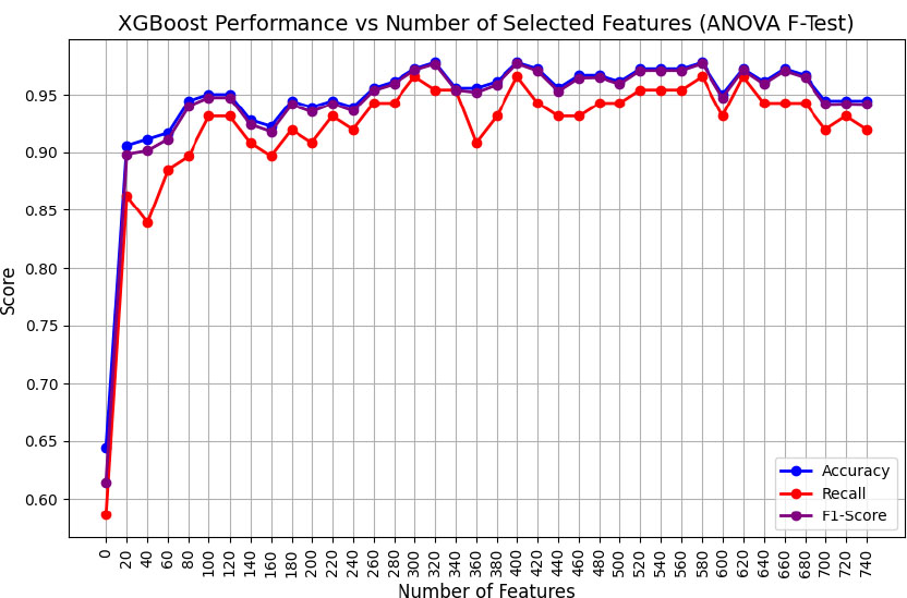
Performance of XGBoost vs. the number of features with ANOVA.
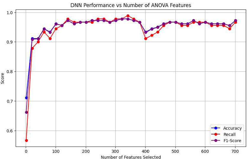
Performance of DNN vs. the number of features with ANOVA.
| Parameter | Value |
|---|---|
| Scaler | StandardScaler() |
| Classifier | SVC(kernel='rbf', max_iter=200) |
| Optimal Features | 300 |
| Training Time (seconds) | 12 |
| Parameter | Value |
|---|---|
| Scaler | StandardScaler() |
| Classifier | XGBClassifier(use_label_encoder=False, eval_metric='logloss') |
| Optimal Features | 320 |
| Training Time (seconds) | 95 |
| Parameter | Value |
|---|---|
| Scaler | StandardScaler() |
| Classifier | MLPClassifier(hidden_layer_sizes=(100, 50),max_iter=500) |
| Optimal Features | 100 |
| Training Time (seconds) | 52 |
CONCLUSION AND FUTURE WORK
As per the study conducted, 90% of the people with Parkinson’s disease suffer from speech and voice-related disorders, based on which speech was found to be an effective marker in the detection of speech. In this study, prominent features from the speech signals were considered, which were applicable to the prediction of Parkinson’s disease. The features considered were shimmer, jitter variants, noise-to-harmonic ratio, pitch period entropy (PPE), and recurrence period density entropy. Spread parameters were found to be important in identifying the disease. For classification, Deep Neural Network yielded a constant accuracy value, leading to the approximation of 78%. In this study, Parkinson’s disease was detected by adding dominating features for over 300,000 voice samples. The existing system gave high accuracy for the small size of the dataset with fewer dimensions. So, the system can be developed for large datasets with more dimensions to detect Parkinson’s disease with improved accuracy and for more voice modulations considering different datasets and features by using a variety of models.
The high-level biological and signal processing features mentioned in Table 1 correspond to a large number of statistical features in the dataset. However, the speech-based benchmark datasets available suffer from insufficient instances for an AI algorithm to generalize. This necessitates the creation of a comprehensive new dataset with a large number of instances to explore the effective interactions with the available features.
Moreover, several studies reviewed in the literature highlighted the significance of patient handwriting-based features [30] and MRI scan-based features [31] as effective approaches for disease prediction. Moreover, with the increasing inflation, the treatment costs of the disease play an important role that needs to be minimized while maximizing the treatment efficiency [32].
Even though the results obtained from the proposed work indicate improved disease detection performance while incurring minimal training costs, the features considered from a single domain may not provide a complete picture of the disease behavior, thus requiring multi-modal and multi-objective parameters for holistic rule learning and data analytics towards disease detection and prevention [33, 34].
AUTHORS’ CONTRIBUTION
It is hereby acknowledged that all authors have accepted responsibility for the manuscript's content and consented to its submission. They have meticulously reviewed all results and unanimously approved the final version of the manuscript.
LIST OF ABBREVIATIONS
| PCA | = Principal Component Analysis |
| SMOTE | = Synthetic Minority Oversampling Technique |
| AI | = Artificial intelligence |
| PD | = Parkinson's Disease |
| SVM | = Support Vector Machines |
AVAILABILITY OF DATA AND MATERIALS
All the data and supporting information are provided within the article.
CONFLICT OF INTEREST
Dr. Vinayakumar Ravi is the associate editorial board member of The Open Bioinformatics Journal.
ACKNOWLEDGEMENTS
Declared none.